How To Find Common Data In Different Excel Sheets
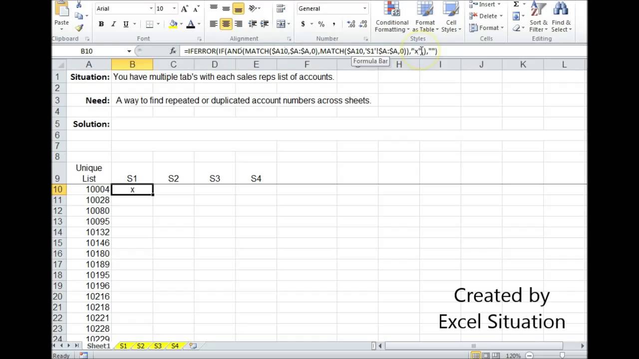
INDEX lookup_table MATCH 1 lookup_value1lookup_range1 lookup_value2lookup_range2 0 return_column_number Note. Name appears in sheet 1 Column A 100 times Dates in sheet 1 Column B from top B6 1-01-2020 B64000 5-01-2020.
How To Compare Two Excel Files Or Sheets For Differences
Now check in both Top Row and Left Column.
How to find common data in different excel sheets. Enter the following code in a module sheet. The other approach uses INDEX MATCH and Excel Table names and references. In the Consolidate dialog do as these.
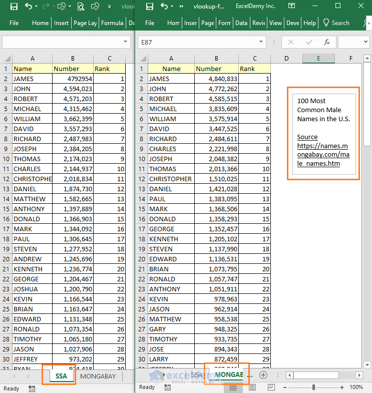
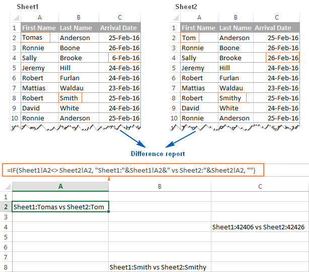
Lets say your data is saved in Sheet1 and Sheet2 of the Excel workbook. In the example shown the formula in F5 is. Using VLOOKUP Formula to Compare Two Columns in Different Worksheets 1 Add a new column Comparing with Mongabay after the Rank column in the SSA worksheet.
There is a dialog displayed on. Locate where you want the data to go. In 1 excel sheet 3 is where formula is to go reference by name is in column A sheet 1 is where to retrieve information from Column A is name Column B is date Column C is Distance so on across 20 columns.
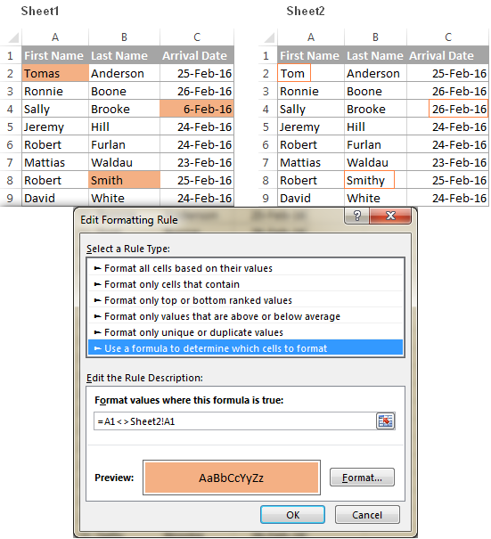
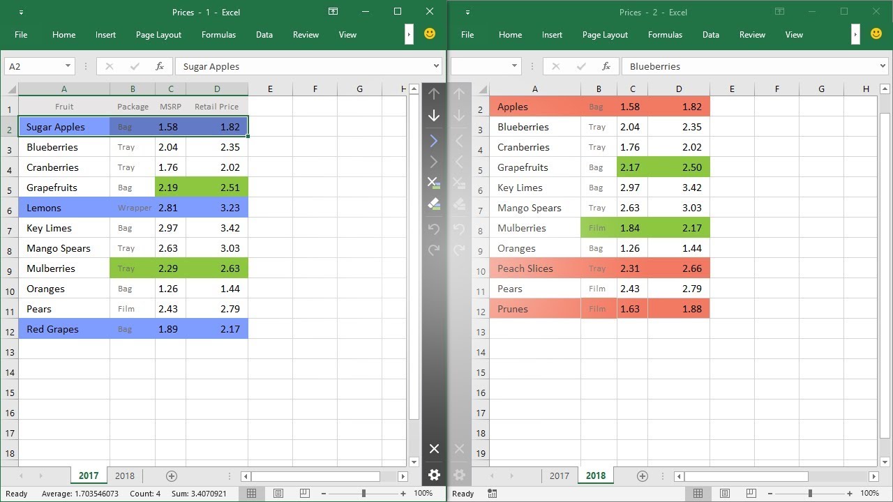
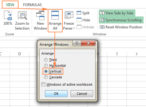
Enable View Side by Side mode by clicking the corresponding button on the ribbon. The key here is that the INDIRECT function acts as the messenger that returns the correct sheet address in a dynamic way to the different lookup formulas. The conditional formatting formula must look for values in matching columns.
Press ALTF11 to start the Visual Basic editor. At the top go to the Formulas tab and click Lookup Reference. Select sheet 1 in.
To compare two lists and extract common values you can use a formula based on the FILTER and COUNTIF functions. Excels vLookup wizard will pop up. Click Insert Module and copy the VBA into the module.
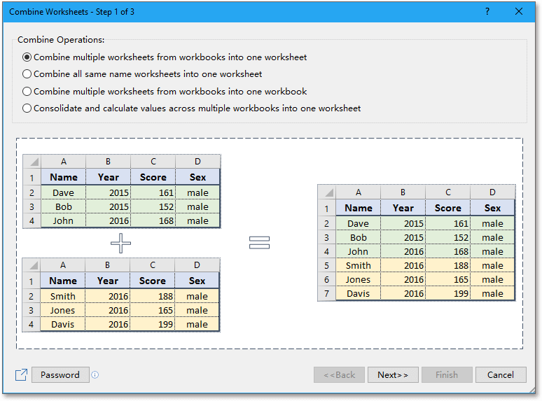
Select the dataset A1. 1 Select one operation you want to do after combine the data in Function drop down list. The matching numbers will be put next to the first column as illustrated here.
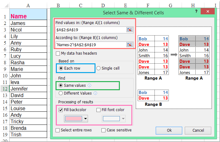
Now select the 2nd range along with Header row and then again click Add. Sub Find_Matches Dim CompareRange As Variant x As Variant y As Variant Set CompareRange equal to the range to which you will compare the selection. You can do both highlight rows that have the same value in a.
In Ref select the first range along with Header row and then click Add. FILTER list1COUNTIF list2 list1 where list1 B5B15 and list2 D5D13 are named ranges. 2 Click to select the range of each sheet you want to collect.
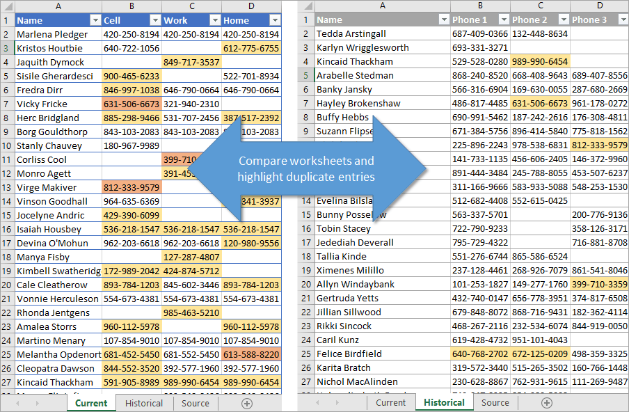
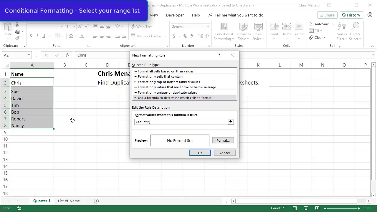
3 Click Add button to add the data range into the All references list box. If the two tables you wish to join do not have a unique identifier such as an order id or SKU you can match values in two or more columns by using this formula. Choose Highlight Cells Rules and then select Duplicates Values in the subsequent menu.
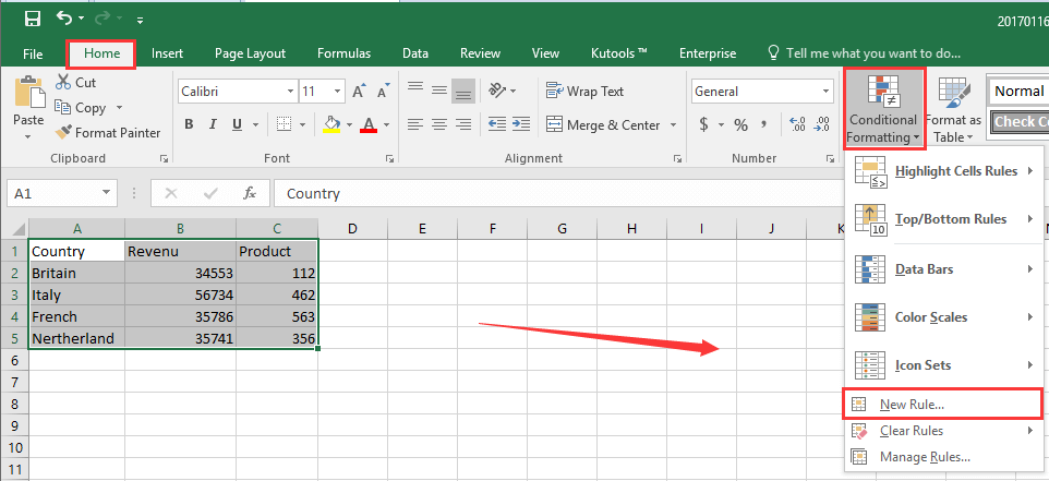
And then input this formula in cell D2. Well walk through each part of the formula. On the Home tab click Conditional Formatting in the Styles group.
Learn how to merge data from multiple worksheets based on a matching key column in Excel without using VLOOKUP functionexcel data merge tutorial. Select the blank single cell where you want your merged data appear. Name by latest date 2nd latest date third latest date.
Click that cell only once. VLOOKUPA2 mongabay_data 1 FALSE. Column B Asset List 1Column C - List 2.
To do this select File Options Customize Ribbon and then select the Developer tab in the customization box on the right-sideClick Find_Matches and then click RunThe duplicate numbers are displayed in column B. In this video tutorial learn how to find matches in two worksheets in Microsoft Excel. How to compare data in two columns to find duplicates.
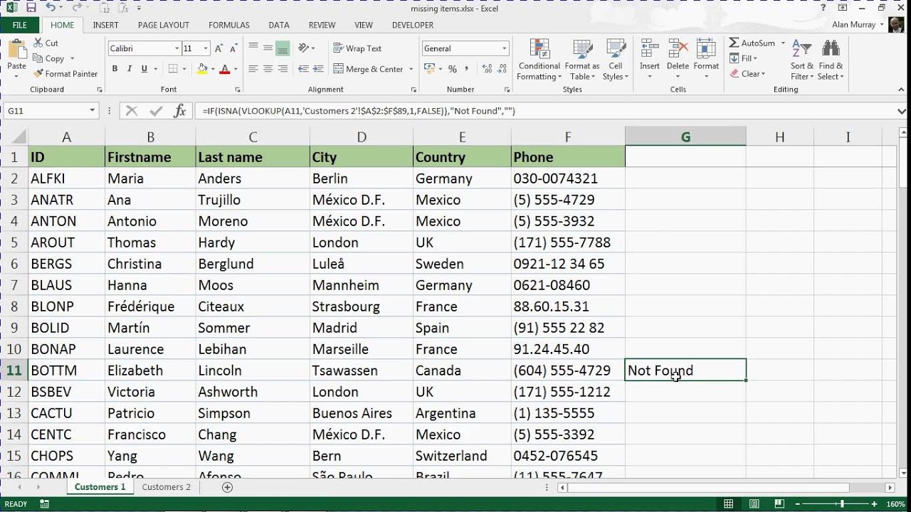
Enter the following formula in cell B1 of Sheet1 COUNTIF Sheet1AASheet2A and Press Enter. In a new sheet of the workbook which you want to collect data from sheets click Data Consolidate. If the record is unique the result will be 0 else the count will tell you how many rows in.
Compare two ranges in two spread sheets with VBA. Highlight Rows with Matching Data or Different Data Another great way to quickly check the rows that have matching data or have different data is to highlight these rows using conditional formatting. A2 is a cell reference to values in column A.
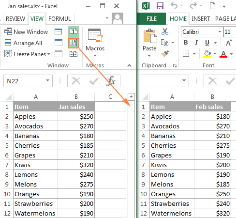
This will open the same Excel file in a different window. List 1Column B - List 2. Column C Cost COUNTIFS YEAR A2 ASSET B2 COST C2 This formula contains absolute and relative cell references.
Click Run button or press F5 to run the VBA. Open your Excel file go to the View tab Window group and click the New Window button. One method uses VLOOKUP and direct worksheet and cell references.
On the Insert menu select Module. Hold ALT button and press F11 on the keyboard to open a Microsoft Visual Basic for Application window.
How To Vlookup To Compare Two Lists In Separated Worksheets
How To Compare Two Sheets In Same Workbook Or Different Workbooks
Compare Two Sheets For Duplicates With Conditional Formatting Excel Campus
Vlookup Formula To Compare Two Columns In Different Sheets
How To Collect Data From Multiple Sheets To A Master Sheet In Excel
Excel Compare Two Worksheets And Highlight Differences Youtube
Excel Finding Duplicates Across Sheets Youtube
How To Compare Two Excel Files Or Sheets For Differences
Compare Two Lists Using The Vlookup Formula Youtube
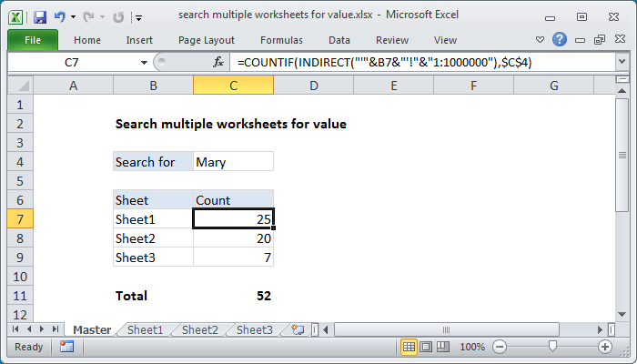
Excel Formula Search Multiple Worksheets For Value Exceljet
Excel Conditional Formatting Find Duplicates On Two Worksheets By Chris Menard Youtube
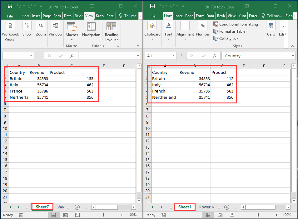
How To Compare Two Sheets In Same Workbook Or Different Workbooks
Excel Find Matching Values In Two Worksheets Tables Or Columns Tutorial Part 1 Youtube
Find And Remove Duplicates In Two Excel Worksheets

How To Compare Two Sheets In Same Workbook Or Different Workbooks
How To Compare Two Excel Files Or Sheets For Differences

How To Compare Two Excel Sheets For Differences
How To Compare Two Excel Files Or Sheets For Differences

How To Match Data In Two Excel Worksheets Basic Excel Tutorial